Robotics 5: 3151A (the world championships)

This is the fifth and final post on my experience in VEX Robotics. In this post, I’ll focus on how I designed the full AI tech stack that we ran on one of our robots for the VEX AI World Championship.

Here are the previous posts:

• Robotics 1: 315P (Over Under)
• Robotics 2: 315P (High Stakes)
• Robotics 3: 3151A (what makes VAIRC difficult?)
• Robotics 4: 3151A (the first competition)

This is a technical post. There’ll be three parts:

• a (very long) explanation of the process we used to write the code that ran on our Jetson Nano compute;
• a walk-through of the relatively short codebase we ran on the VEX V5 brain to talk to the Jetsons;
• and a brief discussion of how we actually performed at the world championship.

Jetson code (notebook excerpt)#

This is an excerpt from our Engineering Notebook, which contains a detailed explanation of our thought process for the architecture. Much of this was dictated at ~11pm sometime in May, so sorry about any typos!

If you just want to see the cool demo, jump to the video!

---

Date: 5/17/2025

Written by: Aadish Verma

General areas#

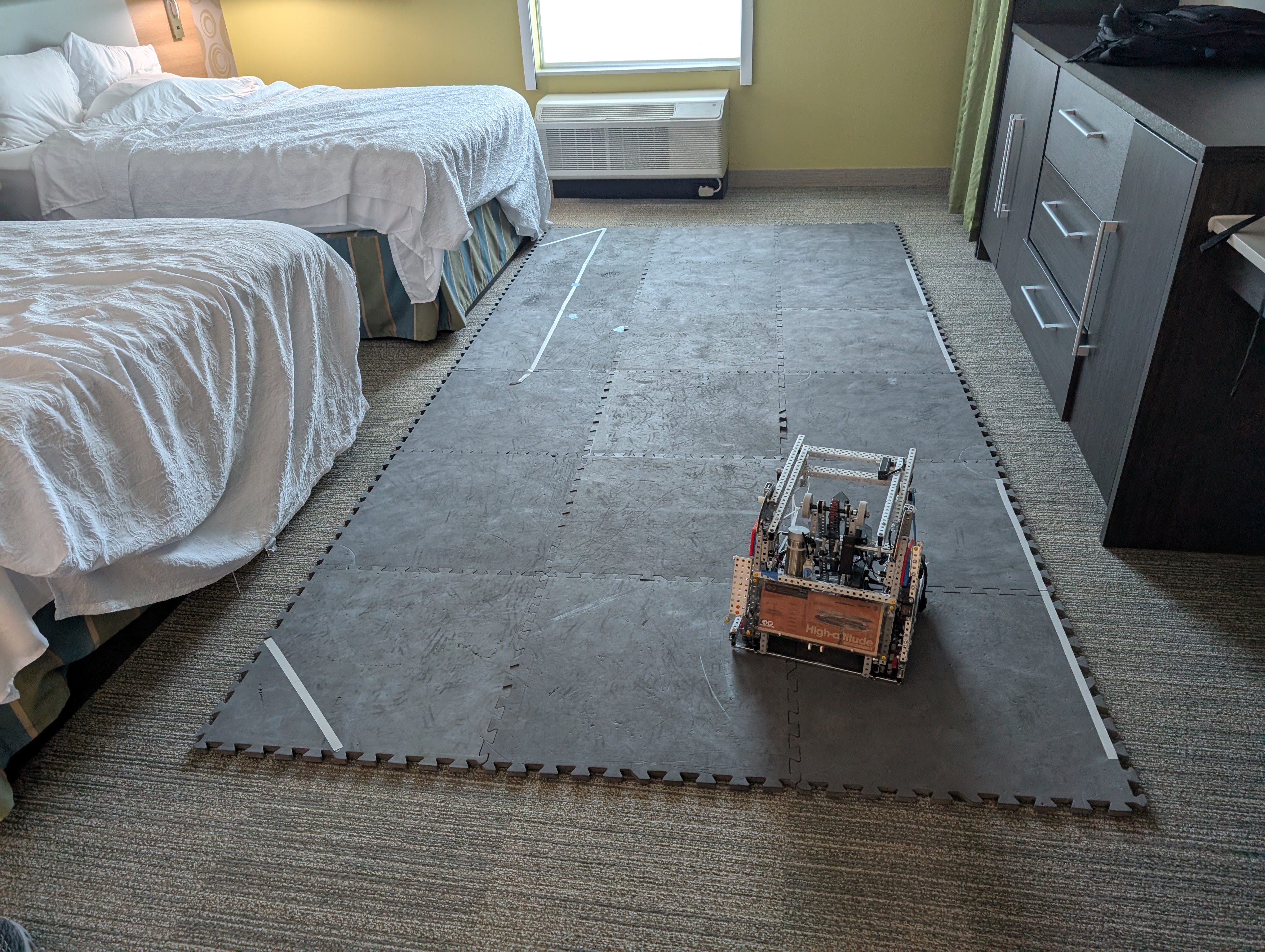
The prominent feature of the VEX AI Robotics Competition is the Interaction Period, in which teams utilize advanced technologies and strategies to interact with field elements and other robots entirely autonomously. For the Interaction Period, 3151A has obtained two NVIDIA Jetson Nanos, which both have powerful GPUs to run neural networks as well as active cooling sufficient to last the 2 minutes of a standard VAIRC match. There are many general areas which we need to consider for the Jetson, which we’ll then refine into more focused subtasks:

Area 1: Detecting objects#

In order to efficiently compete in the interaction period, we need to be able to detect and move to rings on the field. There are numerous methods for this, such as color blob detection (used by the VEX Vision Sensor), or using a neural network (used by the VEX AI Vision Sensor and the VEX AI Image).

After considering both approaches, we decided to go with the neural network. While color blob detection would be simpler, we decided not to use it because it had the potential to be easily tricked, such as if a robot had a license plate the same color as a ring, or the alliance stakes.

The VEX AI image provides a pre-trained YOLO v3 model for use with it. This model is trained on many images from simulation. However, we decided to not use that model for several reasons.

• Choosing to use the VEX AI model would require us to shift into the ecosystem of the VEX AI code, which we were not willing to do as we were planning to write a lot of custom code on the Jetson side.

• After testing the model, we decided that its performance was not up to par. It was only able to run at around 10 frames per second, and it only used the ONNX runtime for the NVIDIA GPU on the Jetson. It did not use the full potential of the TensorRT runtime which NVIDIA exposes, which would significantly speed up the model execution.

• We also found that the model’s quality was not very good. It was not able to detect rings that were less than 10 inches away or more than 40 inches away. At the same time, its detection of mobile goals was terrible, so we could not implement a goal-stealing strategy in our interaction. Similarly, it was only confined to three classes, red ring, blue ring, and mobile goal, which did not include the capability to find robots. This means we cannot detect opponent robots to use for our strategy.

• Finally, the model architecture used also severely limited both performance and quality. YOLO v3 is a relatively old architecture for the YOLO family of object detection models. This is one of the primary reasons that the model’s quality was not as good. When we decided to train our own model, we used much more modern YOLO models for the provided hardware.

Based on this, we decided to train our own custom YOLO model for use with our Jetson Nano. This came with many challenges, however, which we divided up into subtasks.

• Which of the YOLO versions to use, and which model from that specific family to use. Each YOLO family offers multiple sizes of models ranging from nano to large.

• How to efficiently run the models on the Jetson’s GPU using the TensorRT runtime. The YOLO models use a post-processing step known as non-maximum suppression, or NMS for short, which requires a lot of heavy operations. However, this is not built into the YOLO models, meaning that we have to find a way to efficiently execute it either on the CPU or GPU. Also, the YOLO repository, which is generally used for training, exporting, and running YOLO models, is confined to Python 3.8 or above, which does not run on our Jetson Nano. We went through several attempts to install separate Python versions, such as Python 3.8 or Python 3.12, on our Jetson Nano, but none of them were able to detect the CUDA GPU.

• How to efficiently find training data for our models. Object detection models like YOLO require hundreds of images of training data to be able to effectively detect objects. However, finding all of these ourselves and labeling them manually was not ideal as it would require an immense amount of manpower and take time away from other operations of the team. We went through multiple iterations to try to find the optimal blend of manually labeled, publicly available, and AI labeled training data.

• How to access the Intel RealSense D435 cameras that we have obtained for use with the Jetsons. Intel offers a RealSense2 SDK for use with Python. However, we had to find a way to efficiently share the data across multiple different processes that accessed both the depth and color feeds. This was also part of our code architecture subtask. Another big issue was frame alignment. The stereoscopic depth images and the color RGB images from the RealSense are not natively aligned. The RealSense SDK offers a method to align them, but it requires a lot of heavy operations on the CPU and would starve our scheduler of other processes doing work. So we had to find a way to implement a custom alignment process.

• Converting the poses of the detections. While the native output of the V5’s YOLO model after post-processing and NMS are bounding boxes with x, y, width, and height, those do not automatically translate into field coordinates for the VEX High Stakes field. It would require advanced geometry including matrix transformations to bring it from the RealSense’s world space into the robot’s world space.

Area 2: Localization & collision detection#

Most VEX teams use an odometry system including two tracking wheels mounted perpendicular to each other and an IMU to detect orientation changes to properly localize their VEX robots. This works extremely well for the 15-second V5RC autonomous period and the 45-second VURC autonomous period, but for the full two minutes that our robot is needed to be autonomous, this odometry system is likely not feasible. We decided to move forward by testing the “drift” of our current, tracking wheel + IMU-based odometry and seeing how accurate that was.

However, we decided to have a fail-safe Jetson localization method, just in case our drift on our current odometry system was too high. Currently, we have implemented this method to just echo the same pose as is sent over from the V5 brain. However, if needed, we could implement more complex localization algorithms, such as Monte Carlo localization, if we determine that the V5 odometry is not up to standards.

Also, we currently are at risk of getting disqualified for pinning if we run into another robot during the interaction period. We currently need a way of detecting if another robot is immediately in front of us. Currently, we can stop if we run into a robot using a timeout in our motion control library, but if the robot has no other way to escape, that will still count as pinning and disqualify us. We couldn’t just use a front mounted distance sensor, as it might also trigger for ring stacks or rings or mobile goals.

After brainstorming a number of ways to do this, we decided that using the tools we already had was actually ideal. The Intel RealSense camera we were using has a depth mode. So by reading from one row of the depth mode and taking the 10th percentile of the depth value, we can detect if an object is less than 12 inches away from the robot and brake accordingly. We also mounted our RealSense camera so that its center row of measurement was above the plane of any ring stacks, rings, or mobile goals, ensuring that there wouldn’t be any false alarms from field elements. However, implementing this feature was actually relatively difficult, as it required sharing our depth data between our camera process, our inference process, and our collision detection process.

Area 3: Communicating with the V5 Brain#

Since we cannot directly drive the V5 hardware from the Jetson, we have to communicate all of our findings back to the V5 brain. This requires multiple steps. First of all, we need to set up an actual serial connection between the brain and the Jetson using a specified protocol. Then we need to specify a specific way to send packets of data back and forth, as well as a standardized format for reading and writing. Finally, we have to work on reducing latency to ensure that updates from the Jetson arrive at the V5 and are parsed as quickly as possible.

After analyzing the requirements of the above two areas, we decided that there were three main things that we needed to send from the Jetson into the brain:

• The current pose of the robot. As previously noted, we are currently echoing back the same pose that the V5 brain sends, but eventually we may implement more complex algorithms here.

• A list of detected objects. We unfortunately cannot send over the raw data from the inference engine, as after running non-maximum suppression we still need to filter for confidence, convert class indices to class names, and convert camera world space to the robot world space before having a sensible data format to send over to the brain.

• A flag parameter. Currently this parameter can either be an empty string or it can be an all caps STOP. Eventually we might add more modes into this flag parameter but for now this will do. The STOP flag is triggered whenever the collision detection deems an object to be too close to the robot.

A second concern with this is how we’re able to debug the Jetson code. Obviously, there will be inevitable errors with our code, and we need to be able to see exactly what’s going wrong with our inference. This means we need to have some kind of web-based dashboard system which we can access over the network that fetches data from the Jetson and visualizes this in an easy-to-understand manner.

Unfortunately, we cannot just reuse the same code as the Jetson sends to the V5 brain, as there is much more information that we need to debug on the Jetson side, such as the thermals of the Jetson, the camera world space coordinates, etc. This means that the Jetson actually needs to simultaneously create two separate data feeds. The first one is an extremely detailed dashboard feed, which includes basically every single thing you’d want to know about the Jetson as it’s running. The second is a much more filtered version of that feed for the V5 communication, which only includes the relevant data that the brain needs to know.

Completing subtasks#

Based on our brainstorming for the above general areas of concern, we have developed a detailed list of tasks which we will iterate on to achieve our final product. In order to identify the best solution for each, we use the Engineering Design Process. First, we brainstorm a general solution. Next, we research feasible implementations, choose one to move forward with, and implement it. We then test the implementation. If the implementation does not match our standards, we start a new iteration and try a different implementation.

Code architecture#

The issue#

The Jetson codebase is a behemoth and we have rewritten it several times in our quest to find the perfect code architecture. Because of this, it’s extremely important that we choose the correct method for organizing and communication between our files.

The biggest issue we faced while developing our Jetson code is that different parts of the code need to update at different refresh rates. For example, our inference code needs to update at only around 10 frames per second, as it’s generally waiting for around 100 milliseconds every time for the GPU to finish running our model. However, our post-processing code needs to run at up to 30 frames per second in order to update our inference outputs with the most up-to-date depth information. At the same time, our serial communications code does not run at a fixed frame rate and only updates whenever it gets a new update from the V5. During the initial parts of the program, it is completely idle as the V5 has not yet connected. This meant that running all of our programs as a single while loop that refreshes, say, once every 30th of a second was not feasible and would not lead to a good implementation of our goals.

Iteration 1: Web servers#

Our initial iteration for our code structure involved multiple communicating web servers. In order for this to work, we spawned several separate servers using the Flask library in Python. For example, one of our web servers was called the inference web server. And this continually ran the YOLO model on the GPU. Whenever the model finished doing inference, it would then call another web server known as the post-processing web server. The post-processing web server ran things like non-maximum suppression and post-conversion. Finally, the post-processing server would call the serial server to queue up the most recent update to send to the V5 Brain.

We used this architecture for several weeks in our initial Jetson code work. However, we soon ran into multiple issues with it. The biggest issue we encountered was latency. Because every single process was a web worker running the separate Python thread, they could not share memory or files. This meant that a large amount of data such as the tensor of model output from the YOLO model had to be sent over the network. Because we were using Jetson over a Wi-Fi network, this was incredibly slow, as the router had to serve as a middleman between our competing Python web servers

This meant that not only was the data processing incredibly slow, it also taxed the Jetson’s Internet connection, which might have been needed for other things. At the same time, the time between the inference engine running, it finishing inference, and the final data being sent to the V5 brain, was over three seconds, which was completely not feasible for an interaction period where we only had one minute to do dynamic scoring.

Because of this, we decided to move to another architecture where all of the code was spawned by a singular file and was not transferred ever over the network.

Iteration 2: Processes & files#

Our biggest takeaway from the first iteration was that serving data over the network was exceedingly slow for our use case. Thus, we needed to find a better way to communicate between the different processes while still sharing large amounts of data. Of course, these processes cannot all be in the same file as they all ran at different refresh rates. In order to accommodate this, we moved to another model.

In this model, one file served multiple processes using the sub-processing library in Python. These still serve as independent processes, much like in our web server iteration. However, instead of each one having their own web server, these processes communicate using files. For example, the camera process would save the most recent depth and color images to a file, which the inference process would read from. The inference process would then save the YOLO results to a NumPy file, which the post-processing thread would read from, convert to a JSON format, and then store in another file. Then, the serial process reads from this file, and sends the final data to the V5 Brain.

This was a big improvement over Iteration 1 but was still not perfect. It was extremely complex and was not sustainable to maintain for larger codebases. It was also still relatively slow, as it took a long time to save and read from files. Also, there were generally issues of corruption, as we did not use sub-process locks to ensure that only one process was accessing the file at a time, which meant that a process could read from a file at the same time that another process was writing to it, leading to corrupted data. Implementing best practices for communicating between processes, such as using a lock between the processes or using a shared memory library would be exceedingly complex, requiring us to manage the memory ourselves, which would be no better than a language like C++. Because of this, we decided to move off of the multiple process model, as we found that the massive amount of data that we were transferring made this model just not feasible.

Iteration 3: Threads#

After our learnings from the previous two iterations, we decided to move to a model using threads. Threads are superficially the same as processes, but they are actually two distinct things. Processes are entirely separate commands, and are managed by the operating system level scheduler. However, threads are subtasks of the same process and are managed by the Python scheduler, in this case, using the global interpreter lock (GIL). While it seems like our requirement of having multiple separate threads with different refresh rates makes it impossible to use a single process, this is actually perfectly fine for our use cases, as essentially all of our processes spend most of their time idle.

The inference code, for example, spends its time idle waiting for the GPU to finish running the YOLO model. Our serial code spends a lot of its time idle waiting for a response from the V5 brain. The camera thread spends a lot of time waiting for the next frame from our Realsense camera. In this way, most of them actually are not using the CPU for much of their runtime, and thus can release the global interpreter lock during those times, since they are only accessing peripherals. At the entry point of our main.py file, we initialize our subtasks each using the threading library in Python. Then we start them each in parallel and register a shutdown task to cleanly stop them all and release used memory if there is a sudden termination of our process. This makes it incredibly easy to run and debug multiple threads at the same time.

Also, these threads are all methods on the same app instance. This means that they can access global variables on the app instance, allowing them to share memory. This also completely avoids the issue of data corruption. Given the idea of a process, only one thread is using the global interpreter lock, GIL, at a time. This means that there is actually never more than one thread running at a time, as is the old analogy about the scheduler struggling multiple tasks, but only ever running actually one at a time, synchronously. This means that only one thread or task can read or write from a file at a time or memory completely erasing any corruption issues.

You can see how this is implemented in our code walkthrough. After testing this for weeks, we found this to be the best iteration that balanced performance and speed.

Model#

Brainstorming#

The core of our VEX AI system relies on our object detection models, which are crucial for our interaction strategy of dynamically finding and scoring rings. After doing a lot of research and comparing different object detection models, we decided to use the YOLO class of models. YOLO stands for “You only look once” and is generally considered state-of-the-art for object detection tasks. It works by drawing bounding boxes on the images based on the detected objects. It uses a fully convolutional architecture, meaning that it actually works on any image size. However, due to the dated runtime on our Jetson Nano, we will not end up using this feature.

Iteration 1: Only Purdue SIGBots training data + V5S#

While the more recent YOLO V11 and YOLO V12 models are extremely good at architecture and are generally considered state of the art, we were unfortunately not able to use them due to the relatively old hardware on the Jetson Nano, limiting its compute capabilities. We ended up deciding to go with the YOLO V5 class of models. These are relatively old but still well supported for Jetson Nano hardware, and are leaps and bounds better than the YOLO V3 models used by the VEX AI image. We ended up using two of the YOLO V5 family, specifically YOLO V5S and YOLO V5N. These stand for the small and nano variants of the YOLO V5 family, respectively.

Now that the choice of model has been completed, the biggest issue is finding our training data. Training data is extremely hard to find and is the key bottleneck for frontier AI models today. For initial test runs, we decided to use data from the Purdue SIGbots, who run a VEX AI team 1869P. We also found a source from the VEX-U team in China named XJTU1. This source was relatively well labeled and also had many mobile goals labeled. So we decided to use the China based image, if was needed for a better mobile goal detection. For initial runs, we only used the Purdue SIGBots data to speed up our training. If need, we may also add some of our own custom data collected from the robot and phone cameras.

We imported and labeled all of our images using the Roboflow website. This is a very common website for computer version tasks and is used by the Purdue SIGbots as well as XJTU1. Roboflow provides excellent options for post-processing, augmenting, and exporting your dataset. We specifically use it to export a dataset to the YOLO V5 model format. Afterwards, we import it into a Google Colab notebook provided by Roboflow to train our YOLO V5N and YOLO V5S models. We then use the built-in Roboflow mobile detection feature to quickly test the quality of the model on our phones. If we deem the quality excellent, we then transfer it onto the Jetson Nano using the method described in our running the model section to test its performance and speed.

For this first iteration, we decided to train a YOLO V5S model. While it’s relatively bigger, we’ve seen people able to get relatively high frame rates on it with the Jetson Nano. And it also seems to be extremely high quality. So we began training it using the YOLO V5 repository on our Google Colab, the Purdue SIGbot’s training data, and the V5S weights. After importing it into our TensorRT runtime and testing it on the Jetson Nano, we found excellent performance for rings. However, it was incredibly slow. After an incredible amount of optimizations, we were only able to get it running at around 9 frames per second.

While we had shown our pipeline in general worked, we had found three main areas where our model was lacking. The first was speed. Even using the optimized runtime Nvidia provides for our Jetson, we were unable to attain high frame rates. The second was overall quality. While we were generally able to identify most rings in well lit environments, this failed at environments with low lighting, or those with mobile goals in them. The Purdue SIGbots set also included a robot class, which we were not planning to use, but still used for evaluation. Unfortunately, our most recent YOLO V5S model was terrible at detecting robots. The final issue was that all of the model’s detections, regardless of their quality, were incredibly low confidence below 0.2. This meant we could not do confidence-based filtering to get the best, highest quality detections from the model.

Based on our learnings from this iteration, we decided to address these issues one at a time.

Iteration 2: YOLOV5N model + Purdue training data + 300 epochs#

For our second iteration, we decided to address two of the issues at the same time. The first issue, extremely low confidence, would be countered by increasing the amount of epochs or iterations we are training our YOLO V5 model four. We increased this from 99 iterations to 300 to maximize the training. The second issue, speed, would be addressed by changing the model from the YOLO V5 family we were using. For our first iteration, we used a YOLO V5S model, which was good on quality but had extremely low speeds. We decided to switch to a YOLO V5N model, which boasted up to 50% to 100% performance gains in terms of speed, and hopefully not too much of quality drop. All other aspects of our training remain the same.

After testing this out, we found that our confidence was extremely increased up to above 0.5 for the most good detections, and our sensing for mobile goals and robots was significantly improved. Secondly, our speed was also much, much better. We were averaging around 15 frames per second, and with optimizations could often get up to 20 frames per second on our Jetson Nano, especially with improvements like active cooling or other improvements documented in our running the model section.

However, the models still do not perform up to par on mobile goals or robots. Because of this, we decided to add more training data in our next iteration and train for even longer to ensure that we can absolutely maximize the gains in our training and make the V5N models perform as well as possible.

Iteration 3: More training data + 1000 epochs#

With the knowledge of our previous two iterations known, we decided to go for one final attempt to improve our quality on mobile goals and robots. The key change here was to add much, much more training data. With this change, we approximately doubled our training data, from 200 images from the Purdue dataset to a total of 400 images. A hundred of the new images came from the XJTU1 Chinese VEXU team’s images, and another 100 were custom shot from our team, either from the RealSense camera mounted on our robot, or from our phone cameras at home.

Each of these new images was meticulously hand labeled by a human labeller on the team. We also utilize Roboflow’s AI assist features to utilize our previous YOLO V5S model to help us get a good starting point for our labeling. After about three days and immense effort from the team, we were able to fully label the 200 images, augment them, and export them to the YOLO V5 model format. We then trained them for a total of 1,000 epochs or iterations. This was to ensure that the V5N model could internalize as many of the patterns in the data as possible. However, the auto-exit feature of the train script on the YOLO repository actually triggered. This meant that it detected that there was no considerable improvement in the model’s performance after around 500 epochs, so it early exited to avoid wasting resources. This was fine for us as it ensured that we spent as much time as possible and that the YOLO V5 model was unlikely to further improve.

Because of the intense training we were doing for up to 500 epochs, we spent a total of $10 on Google Colab Compute Units to access incredibly powerful graphical processing units or GPUs for our use in training the models. So this was indeed a great investment as even 100 epochs was only a few cents on Google Colab. So we ended up not even fully using our computing, as we still have around 95 units left for use in training future models.

After uploading and testing this final YOLO V5N model, we found that everything about it was completely excellent. Its quality was good on red rings, blue rings, mobile goals, and robots, and it was easily running at a smooth 15 frames per second, and often up to 20 frames per second on our Jetson Nano with a fan on. Based on the massive gains we saw, we decided to make this our final model so we could focus on other things.

Running the model#

Running our model is one of the most important parts of our AI system. Obviously, we need a way to run the model efficiently using the GPU on our Nvidia Jetson Nano. Luckily, there are several open-source attempts to run YOLO models, which of course are very popular on NVIDIA hardware.

There are multiple different methods we explored. They generally fell into one of several classes. The first one is the runtime on which the actual model was executed. This may be the cloud runtime on a server sitting in a data center, the GPU or the CPU. The second is the Python kernel which these libraries ran in. This could either be Python 3.6 or Python 3.8.

To install Python 3.8, we used the pyenv tool. This enables us to install and manage multiple separate versions of Python. For our first two iterations, we set Python 3.8 to be the default Python runtime after installing it to make it easier to run and test code with. We also set pip to default to the Python 3.8 pip version.

We also built a specific evaluation benchmark to test the performance of our models on. This involved running the models on 20 separate images to detect how long it took on each one. Based on this, we calculated an image per second number. We used this both for the technical inference speed of the models themselves, as well as the inference speed of our implementations to run the models on the Jetson Nano. Here are the final eval outputs for each iteration:

• Inference package + CPU: ~3 fps

• Ultralytics SDK + CPU: ~4 fps

• Custom GPU code (Ultralytics NMS): ~0.2 fps

• Custom GPU code (custom NMS): ~15-20 fps

Iteration 1: Inference package + CPU#

We first tried using the officially supported method for Roboflow, which involves uploading our final model to Roboflow. Then we create a Roboflow API key and copy our model ID. On the Jetson side, we can simply import the Roboflow inference SDK, give it our API key and model ID, and pass it images to run on.

This ended up working extremely well for basic testing. However, the vanilla Roboflow inference SDK only supports CPU inference, which would only run at around 3 frames per second on our Jetson Nano.

To install the inference GPU SDK, it requires the ONNX runtime for GPU. The key issue with this, however, is that we are currently using a Python 3.8 as the Roboflow inference SDK has some dependencies that are only available in Python 3.8. However, ONNX Runtime only supports GPU on Python 3.6 since, as previously noted, Python can only detect a Cuda runtime if running within a Python 3.6 environment. This essentially barred us from using the Roboflow inference GPU SDK or the ONNX Runtime for the GPU.

We tried several other methods to get the inference package to load. This included running Python 3.8 in a Docker container, or upgrading our Ubuntu version from 18.04 to 22.04. Unfortunately, none of these worked, or were able to detect the CUDA runtime on our GPU. We decided to try other methods and packages on Python 3.8 to see if they were able to detect our GPU. This way we can identify the root cause of our inability to have the GPU detected on Python 3.8, whether it was a specific issue with the ONNX runtime or if it was an issue with the kernel as a whole.

Iteration 2: Ultralytics SDK + CPU#

The officially recommended way to run YOLO models is the Ultralytics YOLO V5 GitHub repository. It uses PyTorch instead of the ONNX runtime to run the YOLO models, giving us hope that this would be able to detect the GPU on Python 3.8. Unfortunately, you cannot run this on Python 3.6 and guarantee that it will detect the GPU because the Ultralytics repo also depends on some Python 3.8-specific packages.

We already used the ultralytics repo on our Google Colab to train and export the models. We decided to try using it on the Jetson Nano as well, as it contains a “detect” script that efficiently executes the model on provided hardware. We hoped that even given our Python 3.8 runtime, it would be able to detect the GPU and run our model there.

Alas, after installing it and trying to run a basic detection, we found that you still unable to detect the GPU and thus defaulted to running the model on the CPU. This was terrible for us, as it would prevent us from getting any significant speedups over the first iteration.

Based on these learnings, we decided to completely write custom inference code, taking an export of model weights and running it efficiently on a GPU using a Python 3.6 environment, which we already knew is able to detect the CUDA runtime. However, running the model itself, of course, is only part of the story.

After getting the results back from the GPU, the output tensor is not actually immediately workable with bounding boxes. You first have to pass them through non-maximum suppression, or NMS, for post-processing before they’re usable. We decided to simplify our custom implementation by copying over the Ultralytics implementation of NMS into our code. This saved us a lot of coding time; however we would eventually replace it in the future with a simpler implementation for our needs.

Iteration 3: Custom GPU code#

We first spent a lot of time looking into alternative ways to export and implement our YOLO model. The first one is using the ONNX runtime, which the VEX AI image uses in order to achieve lightning fast speeds with the YOLO V3 model. We hope we would be able to get comparable performance using our V5N model.

Another way is Nvidia’s TensorRT runtime, which is specifically designed to enable the maximum amount of acceleration using CUDA and the video processing course on our Jetson Nano.

After benchmarking both options, we found TensorRT to be significantly faster. We suspect this is because TensorRT has some internal optimizations that only NVIDIA is able to do so efficiently. In any case, we decided to move forward using TensorRT for our final custom implementation.

This actually was having to do three separate expert steps. After training our model in Google Colab, it produced a .pt file of weights. “.pt” stands for PyTorch, which is the library that the Ultralytics repository uses to train our YOLO V5N model. However, we cannot directly import this file into PyTorch as it did not contain the necessary model definitions. And PyTorch would not let us run it, obviously, without the correct model definitions. The Ultralytics repository provides these model definitions, but it only runs on Python 3.8, meaning we cannot utilize those. This meant we need to convert the .pt file to another format to run it on our TensorRT runtime.

After training and exporting our .pt file, in the same Google Colab that we used for training, we first of all ran the Ultralytics repository export.py script to convert it to an ONNX file. This ONNX file was sent over to the Jetson Nano. We use secure copy or SCP to do so over the network.

On the Jetson Nano, we ran the trtexec command to convert this to a .engine file, which is the format that TensorRT uses, which is extremely optimized for the specific GPU. This means that we could not run trtexec on the Google Colab, as it would optimize it for the Colab’s GPU instead of the Jetson’s. Then our .engine file is imported into a script which uses the TensorRT Python bindings to load it in, create an engine and run the model.

As noted above, the TensorRT runtime, unfortunately, is only half the story. After that, we use the Ultralytics code to do NMS on the output tensors to use with other algorithms. After importing the Ultralytics code, however, we found that it used some Python 3.8 specific language features. So this meant that we’d still have to run it on Python 3.8. Luckily, this was the first iteration of our code architecture, where we were using multiple web servers. The advantage of this was that we could run the TensorRT code in Python 3.6. This achieves maximum performance, while still running the Ultralytics code on a Python 3.8 web server. This enables them to both communicate over the network protocol, while the intermediate output is saved to a NumPy file (.np).

This worked relatively well for us, but as noted in our code architecture section, this was exceedingly slow for our use case. Most of the time was actually spent sending over model outputs and pinging the Python 3.8 web server. This itself took around half a second. Furthermore, the Ultralytics code was not optimized for our specific model, meaning that it itself also took around one second to run. This actually led to slower performance than our initial CPU implementation. In order to fix this, we decided to completely rewrite our post processing layer to completely speed up the communication with TensorRT and NMS, as well as speed up the NMS itself.

We’ve killed two birds with one stone by using a NumPy implementation of our NMS. Using vanilla NumPy and no external APIs allows us to run on Python 3.6 which means that we could completely ditch the network communication there, and have the two pieces of code directly communicate within the same process. This dramatically sped up our communication times. At the same time, writing it ourselves in raw NumPy was optimized for our model and thus also let it have faster NMS times. Overall, this roughly decreased the amount of time it took to process one image by 10x. After looking through the results, we found that no significant drop in quality was noticed, meaning that we had basically obtained this improvement in speed for free. Because of this, we decided to make this our final inference iteration and move on to the next section of our tasks.

Accessing the camera#

Accessing the camera was actually a little bit harder than it seemed, as this actually required doing multiple things at once. First of all, the color and depth images are not aligned out of the box, so we had to implement our own custom camera aligning algorithm or use a library to do the aligning for us. Secondly, up to three different processes needed the same image data. Saving the images in the file was exceedingly slow as noted in our code architecture section. Luckily, also noted in the code architecture section, our final code architecture allowed us to share memory and variables across separate threads, meaning that that part of the work is actually entirely done for us.

Intel exposes a PyRealSense 2 SDK with Python bindings to use the RealSense camera outputs in our Python code. This dramatically simplified our process of fetching images from the camera. We used the same resolution for color and depth, as well as running at 30 frames per second, which is around twice as fast as our model inference speed. We made it faster than our inference speed so that we could actually update the depths of the most recent predictions faster than the predictions actually changed. This enabled us to do have more fast updates, even if our inference wasn’t up to that speed.

After these realizations, most of our model iterations focused on how to efficiently do alignment.

Iteration 1: Built-in align API#

The PyRealSense 2 API provides a built-in method for aligning the color and depth frames using focal length and other intrinsic properties of the camera to effectively align them every frame. We use this in our initial implementation to extremely simplify our code.

However, when using this code, we noticed a weird behavior with our inference thread. The inference thread only seems to be updating the detections once every fourth of a second, even though we knew based on our evaluations that the model itself could easily run at up to 20 frames per second. We decided to debug a lot, and after installing several debugging tools to visualize how much time each thread is using per second in our process, found that the PyRealSense2 align API was actually the issue.

The aligned code seems to be calling a lot of loops in the underlying C++ code. While being C++ code, it’s still extremely fast, having to loop over every pixel in the image and do an computationally intensive calculation on them uses a lot of CPU time. And because this is still running on the CPU and not as a peripheral, it holds our global interpreter lock or GIL for up to three quarters of a second for every second of the process. This meant that all of the other threads had to compete for the remaining quarter of a second to use for their own code.

This effectively limited many of our threads to run for only three or four frames per second. This actually held us up for up to a week because we were seeing mysterious slowdowns in other parts of our code. We never realized that our align API was actually blocking the process for so long that these threads were actually being starved of their execution time.

Iteration 2: Custom align#

Based on these learnings, we decided to create a much more optimized align API, since these computationally intensive computations were not only easily parallelizable on the GPU, but were also approximately the same every time, meaning we could actually express them as a matrix multiplication, which is of course much simpler for libraries like NumPy to execute.

Our initial attempts involved using Jax, which is a NumPy equivalent that runs computations on the GPU to do our alignment. This worked relatively well, but for some reason JAX did not detect our GPU. In order to address this, we decided to switch to a much simpler approach. This involved saving our alignment matrices to a NumPy file instead of dynamically computing them at runtime. This simple change shaved off over 15 seconds from our startup times. We also then use those loaded matrices instead of the PyRealsense 2 SDK’s alignment to align the images. This provides up to a 10x speedup in the time for alignment per frame.

This is enough speed to avoid the GIL-starving issues we experienced earlier, so we decided to let this be our final iteration for alignment.

Another issue we had was that our lighting conditions were very variable depending on where we were testing the RealSense camera in. To achieve this, we actually created a program that would constantly read from a JSON file which stored offsets to tune our HSV colors, to be in the same color profile regardless of environment. For every different environment that the camera would be in, we tuned the JSON file specifically for that environment. This concluded all of our work for the camera side.

Post-processing model outputs#

Here’s an overview of how our post-processing works:

• Setup

  • Grabs the app, robot’s starting position, and camera info.

  • Sets up some starting numbers and a simple object for finding location.

• Distance check

  • Figures out how far away things are using the camera’s depth image.

  • Looks at the depth in the area around each thing detected.

  • Handles bad depth readings.

• Computer info

  • Tries to read the Jetson’s temperature and how long it’s been running.

• Data conversion convert_to_v5

  • Changes the data to a new format

    • Makes the theta value negative

    • Renames the values

    • Uses json.dumps to convert dictionary to string

• Main update function

  • Grabs the depth image, detections, and robot position.

  • Adjusts what it sees

    • Scales the vertical position of detections.

    • Changes the size of goal detections for some models.

    • Finds the depth of each detection.

    • Ignores detections it’s not sure about.

  • Finding location

    • Converts camera positions to world positions using a special function.

  • Check for obstacles

    • Looks at a line in the depth image for things in the way.

    • Sets a “STOP” flag if something is too close.

  • Builds the report

    • Includes robot position, detections, the stop flag, and Jetson info.

    • Converts the data to V5 json format with convert_to_v5.

  • Returns the report.

Serial layer#

Here’s an overview of how our serial code works:

• Starts communication

  • Establishes a connection to the robot’s serial port.

• Main operation

  • Continuously reads messages from the robot.

  • If the connection fails, it automatically attempts to reconnect.

• Receives data

  • Acquires a line of text from the serial port.

  • Cleans the text.

• Understands the data

  • Attempts to convert the text into a structured data format (like a Python dictionary).

  • If conversion fails, the malformed data is logged.

• Initial setup

  • For the first message received, all position values are used to configure a Processing object.

• Subsequent actions

  • Extracts x, y, and theta position values.

  • Utilizes the update function in the Processing object to determine the robot’s complete environmental state.

  • Converts this state to a V5 format.

  • Transmits the V5 formatted information back to the robot.

• Error management

  • If a problem occurs during serial communication, an error is reported and reconnection is attempted after a short pause.

Terminal forwarding#

Our Jetson serial implementation ended up working great. However, it is often the case that one of our coders for the isolation period needs to debug a specific part of code or API when coding for the robot and the V5 brain. This was previously near impossible. This was because using cout or printf, which are typically used for debugging statements, doesn’t work anymore. This is for two separate reasons.

The first reason is the change in the encoding scheme. We use the PROS framework instead of VEXcode for our programming on the V5 side. PROS uses an encoding scheme known as COBS to ensure that packet delimiters do not include as part of message content. This works great for the PROS integrated terminal, which is what most V5RC teams use to debug their statements, and is what cout or printf log to. However, this is not good for our VEX AI code, because our Jetson serial layer does not handle COBS decoding. Because of this, we actually disable the COBS layer on the V5 side. This dramatically simplifies our serial layer while still allowing us to send data back and forth. This actually speeds up our serial code because the compute of needing to encode and decode using COBS is completely bypassed. However, the code for the PROS integrated terminal assumes that the serial input from the V5 brain’s stdout is using COBS encoding. Otherwise, it fails to correctly decode the packets. This means that even if the packets do end up making it to the computer, they will be read as gibberish.

The second reason is a specific implementation detail of the V5 SDK itself. We send messages to the Jetson over a USB serial connection. We choose to use USB because there are already well-established encoding schemes for doing so, and PROS automatically routes cout or printf calls through the USB port first. However, for some reason, if a USB serial device is connected, it does not also forward those packets to the controller and then to the computer. This makes logging practically impossible, as we cannot view the packets from the controller, and we cannot connect our computer directly to the brain, because the brain USB port is already in use from the Jetson. This means that in all cases, we are unable to receive packets from the Jetson on our computer.

This is a big issue. Much of our team’s work involves tuning small things or checking if there’s a major bug. Both of these require an insane amount of logging. For example, when trying to debug a specific crash, we often need to add print statements on every other line of code. We cannot simply implement these in another way. Similarly, for things like tuning the distance our PID goes or the specific PID values of our motion controllers, we often need to log the error or KP values or our motion controller. It would be much harder to do this without the terminal.

One way to bypass this is to have each process that needs to log something, have its own specific implementation for logging. For example, PID tuning could create its own UI based on the LVGL graphic language, or debugging could invent its own visual debugger for the V5 brain screen. However, this is insanely complex and not feasible for the short term, especially for the smaller logging needs. We decided to then begin looking into ways to so-called “harvest” the data from the brain’s USB connection that is sent to the Jetson in a way that we can route it back to our computers in order to read what it sends.

We ended up implementing this using an event stream. HTTPS or HTTP connections are generally short-lived, where a single request is made and the entire file is sent over immediately. This works for most use cases, such as loading a website or fetching a video. However, some things require continual updates from the server. Because of this, an entirely separate version of the HTTP spec, known as server-side events or SSE for short, was created.

The key idea of SSE is that it is a long-living connection. That means that the request does not terminate immediately after the first response. Instead, the host keeps the HTTP connection open and continually appends updates to the message. You can consider like another version of the serial layer, but instead of going over the USB, it goes over the network. In this sense, the host is continually sending new packets of information to the client.

We actually already used server-side events on our dashboard. To get this to work, we actually created our own custom wrapper of the Flask webserver Library for Python. In this wrapper, the host, or in this case, the Jetson, establishes a long-living connection, and asynchronously yields new appended content to a message. In this case, the content is a JSON blob containing literally everything the dashboard needs to know about the Jetson, detections, and the V5 side. On the client side, we actually are able to use the JavaScript or TypeScript async API to leave the thread idle until a new message is sent from the HTTP host. This is much simpler and more performant than the web socket implementation of the VEX AI dashboard that is built in to the provided image. It’s also much less code since it’s a one-way communication.

We implemented something similar in front of our serial layer for the Jetson. Whenever we receive a new package from the V5, we first of all decode it using UTF-8. UTF-8 is an extension of the ASCII protocol for encoding text which adds support for unicode characters. After decoding successfully, we then attempt to parse the message as a JSON packet. If the message is a JSON packet, we know it was sent from the V5 side of the serial layer, and it contains important information about the robot’s pose and detections. Otherwise, we know it’s something else, such as a log message from another part of the program. Based on this, we route the data to one of two possible places. If it’s a JSON packet, we send it to our post-processing service, which is the key input, which is the key entry point for any and all inputs from the serial layer.

If we deem it to not be a JSON packet, and instead be another part of logging, we actually route it to our web server instance. If you recall, we use our web server for multiple things, such as the color live stream, the depth map live stream, and the asynchronous SSE-based events endpoint.

For our terminal forwarding, we add another endpoint, which continually checks if we have a new log message routed over from our serial layer. If there is, we append it to a web request. This way, one can simply go to the Jetson’s IP followed by a URL in their browser, and the terminal messages will load in one by one in an asynchronous fashion. This is not only a very simple way to get terminal forwarding working, but also completely fixes our team’s problems, as this enables us the exact same surface area for logging as the old PROS terminal did.

It is also extremely fast if we use the Jetson’s access point mode in which it creates its own Wi-Fi network. By combining these innovations, we are able to get an incredibly performant and high-quality terminal forwarding that is not compromised on our serial layer either.

Let’s walk through the code for implementing this: Our App class is the key entry point for any worker on the app:

class App:
    def __init__(self):
        # initializing workers and shared memory
        self.camera = CameraWorker()
        self.inference = InferenceWorker(self)
        self.most_recent_result = {}
...

For the terminal forwarding, we also have an array of strings v5_logs which contain every non-JSON packet received from the V5 since the program was started:

    def __init__(self):
       ...
       self.v5_logs = []

Most of the action takes place in the App.service_serial method, which handles any and all communications with the brain.

    def service_serial(self):
        ser = serial.Serial(...)
        post = None
        while True:
            try:
                if not ser:
                    ser = serial.Serial(...)
                line = ser.readline().decode("utf-8", "replace").strip()
                try:
                    data = json.loads(line)
                except Exception as e:
                    # this data is not a JSON packet
                    continue
                if post is None:
                    post = Processing(...)
                    continue
                self.most_recent_result = ...
                v5_json = post.convert_to_v5(self.most_recent_result)
                ser.write((v5_json + "\n").encode("utf-8"))
                time.sleep(1.0 / 30.0)
            except serial.SerialException as e:
                print("Encountered error in serial loop:", e)
                del ser
                time.sleep(1.0)

Implementing port forwarding is actually a one-line change:

    def service_serial(self):
        ser = serial.Serial(...)
        post = None
        while True:
            try:
                ...
                try:
                    data = json.loads(line)
                except Exception as e:
                    # this data is not a JSON packet
                    # add this line ↓
                    self.v5_logs.append(line)
                    continue
            ...

That’s all you need to start appending non-JSON packets to the shared v5_logs variable!

To implement the web server side we look at our DashboardServer class. This handles all of our webserver-related code. To run the server, you can simply call DashboardServer(App()).run(). (We initialize it with an App instance so it can access the shared memory from the app.)

class DashboardServer:
    def __init__(self, app_instance):
        self.app_instance = app_instance
        self.flask_app = Flask(...)
        self._setup_routes()

    def _setup_routes(self):
        app = self.flask_app
        app_instance = self.app_instance

        @app.route('/<type>.mjpg')
        def video_feed(type):
            ...
        @app.route('/update_hsv', methods=['POST'])
        def update_hsv_config():
            ...

        @app.route('/')
        def index():
            ...

    def run(self):
        ...
        # run webserver on network to be exposed to other clients
        self.flask_app.run(host='0.0.0.0', port=5000)

Let’s add our SSE endpoints for the terminal forwarder (also known as the logger):

    def _setup_routes(self):
        ...
    def run_events():
        # Return at least one line, otherwise the browser is in an indeterminate state
        yield "\n"
        # last_len stores the most recent length of the v5_logs
        # we compare current length of v5_logs with last_len to check for new updates
        last_len = 0
        while True:
            # some Python list magic
            # we basically go through every new log that we haven't printed before and append it to the response
            for stuff in self.app_instance.v5_logs[last_len:]:
                yield stuff + "\n"
                # update last_len
                last_len = len(self.app_instance.v5_logs)
                time.sleep(1.0 / 30.0)
    @self.app.route('/terminal')
    def v5_logger():
        headers = {
            'Content-Type': 'text/event-stream',
            'Cache-Control': 'no-cache',
            'X-Accel-Buffering': 'no'
        }
        return Response(stream_with_context(run_events()), headers=headers)

Now, going to <jetson_ip>:5000/terminal successfully shows an asynchronous, continually updating stream of logs from the V5 brain’s stdout interface. If we run the Jetson in access point mode, the terminal can be found at 10.42.0.1:5000/terminal.

Dashboard#

In order to properly visualize all of our testing, we built a web dashboard to help us simplify debugging.

• Depth Feed — a depth map from the Realsense camera, live stream

This was written as part of a team member’s website. It uses the following technologies:

• React, a JavaScript library for building interactive, component-based Web UIs
• Astro, a Server-Side Rendering framework that React is used with to improve site performance
• TailwindCSS, a styling solution to simplify our layouts
• shadcn/ui, a component library built on top of TailwindCSS that provides good default components (such as buttons and cards)
• React Mosaic, a library for building drag-and-drop, window management-style experiences
• TypeScript, a superset of JavaScript that adds strict typing behaviors to decrease the amounts of errors The dashboard offers a comprehensive experience. It offers multiple views to debug separate aspects:
• Color Feed — a color image from the Realsense camera, live stream
• Raw Data — shows the raw JSON that the Jetson outputs
• Details — shows specific details, such as numbers for detections and thermals + uptime for Jetson
• Field View — visualizes the robot pose and detections on a field image to provide a realistic simulation How the dashboard is hosted is also particularly interesting:
• The dashboard itself is a Bun app with is written in TypeScript.
• The dashboard is run on a team member’s computer. Unlike the Node.js-based VEX AI dashboard for the default VEX code, this dramatically reduces the amount of data coming over the network (as the JavaScript bundle is massive) and improves responsively. The dashboard only exchanges JSON packets with the Jetson, instead of having to reload the entire page when new data is acquired.

Here is a video of the dashboard fully working:

---

And that ends our engineering notebook excerpt.

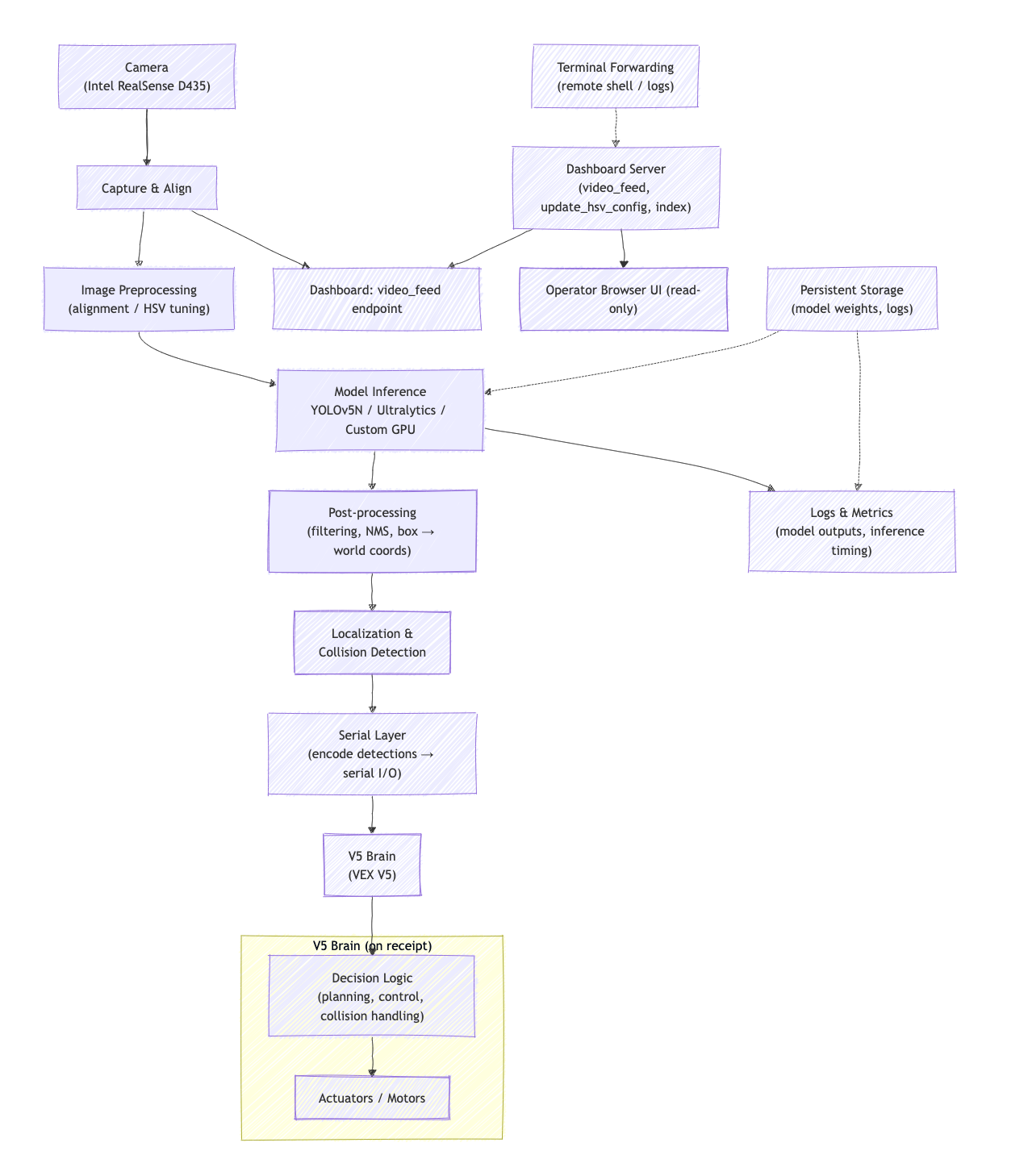
Here’s a high-level overview diagram of our architecture:

V5 codebase#

The codebase we ran on the V5 brain is actually quite simple. Quick reminder:

• We run all compute-intensive tasks on the NVIDIA Jetson Nano, then forward it to
• the VEX V5 brain, which has access to all of our robots’ peripherals (sensors & motors).

All communication is done through USB serial, which is exposed to our C++ code on the brain through stdin/stdout (or cin/cout in C++). Our entire serial communications code is thus very simple, involving mainly just parsing JSON packets. I’ve put in our abbreviated code below, combining the header and code files:

#pragma once
#include "robot.hpp"
#include "jetson.hpp"
#include "nlohmann/json.hpp"
#include "pros/apix.h"
#include "robot.hpp"
#include <exception>
#include <iostream>
#include <tuple>
#include <vector>
#include <optional>
#include <string>

using json = nlohmann::json;
using namespace std;

namespace serial {
    // one YOLO deetection
    struct Detection {
        double x;
        double y;
        double z;
        std::string cls;
    };
    // one JSON packet received from the Jetson
    struct Frame {
        std::string flag;
        std::vector<Detection> detections;
        std::tuple<double, double, double> pose;

        // Checks if a detection is still present in the frame and returns the
        // closest match
        std::optional<Detection> is_present(const Detection &detection) const;

        // Returns the detection with the given class whose (x, y) is closest to
        // (x, y), or nullopt if none found
        std::optional<Detection> get_match(robot::RingColor color, double x,
                                           double y) const;
    };

    // ...I've omitted implementations for `Frame`'s methods since they are
    // relatively trivial

    std::optional<Frame> frame = std::nullopt;
    double last_time = 0.0;


   std::optional<Frame> parseFrame(const json &j) {
       try {
           Frame f;
           f.flag = j.value("flag", "");

           if (j.contains("pose") && j["pose"].is_object()) {
               const auto &p = j["pose"];
               double x = p.value("x", 0.0);
               double y = p.value("y", 0.0);
               double theta = p.value("theta", 0.0);
               f.pose = std::make_tuple(x, y, theta);
           } else {
               return std::nullopt;
           }

           // The JSON uses the key "stuff" for the detections
           if (j.contains("stuff") && j["stuff"].is_array()) {
               for (const auto &item : j["stuff"]) {
                   if (item.is_object()) {
                       Detection d;
                       d.x = item.value("x", 0.0);
                       d.y = item.value("y", 0.0);
                       d.z = item.value("z", 0.0);
                       d.cls = item.value("class", std::string{});
                       f.detections.push_back(d);
                   }
               }
           }

           return f;
       } catch (...) {
           // Catch any parsing errors that might occur
           return std::nullopt;
       }
   }

   std::optional<Frame> fetch_frame() {
       try {
           std::string line;
           if (std::getline(std::cin, line)) {
               json j = json::parse(line, nullptr, false);
               if (j.is_discarded()) {
                   std::cerr << "Invalid JSON received" << std::endl;
                   return std::nullopt;
               }
               return parseFrame(j);
           }
       } catch (json::parse_error &e) {
           std::cerr << "JSON parsing error: " << e.what() << '\n'
                     << "exception id: " << e.id << '\n'
                     << "byte position of error: " << e.byte << std::endl;
       } catch (const std::exception &e) {
           std::cerr << "An unexpected error occurred: " << e.what()
                     << std::endl;
       } catch (...) {
           std::cerr << "An unknown error occurred." << std::endl;
       }
       return std::nullopt;
   }

   void task_send() {
       pros::c::serctl(SERCTL_DISABLE_COBS, NULL);

       while (true) {
           auto pose = robot::drive::chassis.getPose();
           printf("{\"x\": %f,\"y\": %f, \"theta\": %f}\r\n", pose.x, pose.y,
                  -pose.theta);
           fflush(stdout);
           // timeout
           if (frame.has_value() && pros::millis() - last_time > 500) {
               frame.reset();
           }
           pros::delay(50);
       }
   }
   void task_receive() {
       pros::c::serctl(SERCTL_DISABLE_COBS, NULL); // for redundancy

       while (true) {
           // ↓ uses regular old `cin`
           frame = fetch_frame();
           last_time = pros::millis();
           pros::delay(33);
       }
   }
} // namespace serial

The key functions to look at are the fetch_frame, task_send, and task_receive; these encode the core of our serial protocol. Note how they all use cin and cout like a normal C++ program would — PROS forwards this to/from the USB port on the brain. The protocol that fetch_frame parses matches the one used in our Python code on the Jetson Nao:

    def convert_to_v5(self, data):
        result = copy.deepcopy(data)
        # Create a new object from scratch instead of modifying the existing one
        new_result = {
            'pose': {
                'x': result['pose']['x'],
                'y': result['pose']['y'],
                'theta': -result['pose']['theta']
            },
            'stuff': [],
            'flag': result['flag']
        }

        # Copy and transform each detection
        for det in result['stuff']:
            new_det = {
                'x': det['fx'],
                'y': det['fy'],
                'z': det['fz'],
                'class': det['class']
            }
            new_result['stuff'].append(new_det)

        result = json.dumps(new_result, separators=(",", ":"))
        return result

The 33 millisecond delay is just to roughly ensure that both the brain and the Jetson Nano operate at 30fps or lower (to avoid packet loss, CPU starvation, excessive computations, etc.). The protocol operates under a “push” system — the brain sends a packet, the Jetson receives a packet, and sends a new packet back to the brain — so our delay for the sending thread (task) is longer than the delay for the receiving task to avoid them getting out of sync.

The line:

pros::c::serctl(SERCTL_DISABLE_COBS, NULL);

might look a bit weird. It basically translates to configure the serial driver to disable cobs encoding, which is necessary. Otherwise, PROS would automatically use COBS to encode our packets which would require us to reimplement COBS decoding on the Jetson Nano. This obviously isn’t ideal!

quick side note: COBS encoding basically ensures our packet delimiter never shows up in the packet contents to avoid ambiguity.

It isn’t super obvious at first why we need two separate tasks for sending and receiving packets. After all, we know that the Jetson only sends us a packet after we’ve sent it one packet. This is what we thought too, at first, so we implemented it as a single task, like so:

    void task_send() {
       pros::c::serctl(SERCTL_DISABLE_COBS, NULL);

       while (true) {
           auto pose = robot::drive::chassis.getPose();
           printf("{\"x\": %f,\"y\": %f, \"theta\": %f}\r\n", pose.x, pose.y, pose.theta);
           fflush(stdout);
           most_recent_frame = fetch_frame();
           pros::delay(30);
       }
   }

This looks like it works, but fails in a specific edge case — when the Jetson disconnects. In this case, the fetch_frame call will hang forever, waiting for the (temporarily disconnected) Jetson to send a packet. The Jetson typically will immediately reconnect after ~100ms, but due to the push system, it waits for a packet from us before it will send us a packet. This leads to a chicken-and-egg problem:

• the Jetson is waiting for us to send a packet, after which it will send us a packet, but
• our fetch_frame call is blocking until we get a packet from the Jetson, after which we’ll send an new packet.

The solution to this is to separate the sender and receiver functions, like we did in the above code. This way, the sender is constantly pumping packets into the Jetson, no matter what the state of the receiver is. This means that, when the Jetson reconnects, we immediately start sending packets again, and the Jetson will immediately send us a packet (and thus allow the receiver to continue). The key thing about this model is that, if the receiver hangs while waiting for a Jetson packet, our sender is not blocked.

That wraps up the discussion of our V5-side code. I would love to show some of the actual business logic that we ran but unfortunately do not have permission yet to share it. In the meantime, you’ll have to make do with this excerpt that provides an example of how we used the Frame methods to control our motions in the Interaction Period:

std::optional<Detection> check_if_feasible() {
    // `color` is a macro which returns the current alliance/side we're playing for
    cout << "[check_if_feasible] color " << (color) << endl;
    // Ensure there's a frame to process
    if (!frame.has_value()) {
        return nullopt;
    }

    std::optional<Detection> initial_match_opt =
        frame.value().get_match(color, chassis.getPose().x,
                                chassis.getPose().y);

    if (!initial_match_opt.has_value()) {
        return nullopt;
    }

    // If a "red" detection was found, work with its value.
    Detection current_best_match = initial_match_opt.value();

    // Filter this initial match based on its absolute coordinates
    // (e.g., too far from field center)
    if (std::max(fabs(current_best_match.x),
                    fabs(current_best_match.y)) >= RING_BOUND_ABSXY) {
        return nullopt;
    }

    // Log the initial detection that passed the first filter.
    cout << "[check_if_feasible] Initial best match is of class "
            << current_best_match.cls << " at point ("
            << current_best_match.x << ", " << current_best_match.y << ")"
            << endl;

    int score = 10;

    for (int i = 0; i < 10; ++i) {
        pros::delay(50);

        if (!frame.has_value()) {
            --score;
            continue;
        }

        std::optional<Detection> updated_match_in_new_frame_opt =
            frame.value().is_present(current_best_match);

        if (updated_match_in_new_frame_opt.has_value()) {
            current_best_match = updated_match_in_new_frame_opt.value();

        } else {
            --score; // penalize confidence
        }
    }

    // If confidence score is still high enough after the confirmation
    // loop, return the (potentially updated) current_best_match.
    if (score > 5) {
        return optional<Detection>{current_best_match};
    } else {
        cout << "[check_if_feasible] we lost it" << endl;
        return nullopt; // Confidence too low, or object lost.
    }
}

Conclusion: our performance at worlds#

We didn’t perform… ideally at worlds, but our goal arguably was never to win. A brief breakdown:

• Won qualifiers 12, 22, 46, 82, 102, 121, 166, and 191. Lost qualifiers 142 and 156.
• Won R16 (octofinals) but lost in quarterfinals.

I don’t want to say too much about the reasons behind our team’s performance since I’m inevitably biased, but concisely:

• We were limiting under an extremely constrained timeframe. The team itself had only really started work <2 months out from the championships, despite most teams having the full competition season to work. Obviously not an excuse, but a majority of the work in all VEX competitions is tuning autonomous routines, which is extremely time-consuming and mundane. We did not have much opportunity for tuning, with robots often alternating between builders’ homes and robots often being in limbo due to hardware issues.
  • This isn’t to blame the hardware team; they did amazing! They fixed issues tirelessly, but the time constraints were all-controlling.
• We were often limited by weird issues with drivers or CUDA versions (many of which are detailed in the above notebook excerpt). This was my first time personally working with advanced custom AI on CUDA systems, so I had to learn a lot about the hardware and software stack. Additionally, we had to deal with issues related to the NVIDIA Jetson Nano, which is a powerful but limited device. All of this took a lot of time to debug and resolve.
• Having three separate teams split across two robots was not at all conducive to our teamwork. I think we could have done better if we had set more realistic expectations and clearly communicated our requirements.

And more broadly:

• VEX High Stakes is innately anti-AI. Obviously, I’m being a bit of a sore loser, but I genuinely believe that the VEX AI competition itself innately is not able to support AI. A double tier 3 hang (don’t worry exactly what that is) could score more points than any AI-based strategy, and can be implemented solely using hardware and a tiny bit of programming. The few teams that did use AI (like us) got a lot of cool results, but just not the points :(
• Despite our not-very-good showing, I’m still very proud of everything we accomplished. We were the only team to use AI in competition to autonomously score a range on a wall stake (tl;dr a nontrivial task to do autonomously), and even scored on mobile goals quite a lot using the AI.
• One of the funniest stories I’ll get from this is why we lost quarterfinals — it was due to a very obscure bug in LemLib, the motion controls library we used, which had a subtle bug which failed to release a mutex, leading to our robot being in a deadlock for the full interaction period (the time where we had expected to score most of our points). This eventually spun into a full-blown issue and associated pull request to fix the critical bug. I’ll hopefully write a bit more about that soon!

Unfortunately, 3151A will not be continuing to compete in VEX for the foreseeable future, but I thank all of my teammates, and the dozens of competitors from around the world, but helping us pull off such a feat in two months.

You can view AIWorlds, our Jetson-side codebase, here. As noted above, I haven’t yet obtained permission to share our V5 Brain codebase, but I’ll update this post once I do.

Thanks for reading!